Clustering in Machine Learning

Clustering is a type of unsupervised learning in machine learning where the goal is to group a set of objects in such a way that objects in the same group (or cluster) are more similar to each other than to those in other groups. Clustering is widely used in data mining, pattern recognition, image analysis, information retrieval, and bioinformatics.

What is Clustering?

Clustering involves partitioning a dataset into subsets, or clusters, where data points within each cluster share common traits or characteristics. Unlike supervised learning, clustering does not rely on predefined labels or categories; instead, it discovers these groups based on the inherent structure of the data.

Applications of Clustering

1. Market Segmentation: Identifying distinct groups of customers based on purchasing behavior.
2. Social Network Analysis: Detecting communities within social networks.
3. Image Segmentation: Dividing an image into segments for analysis.
4. Anomaly Detection: Identifying unusual data points that do not fit into any cluster.
5. Document Clustering: Grouping similar documents for topic extraction.

Types of Clustering Methods: 

1. Partitioning Clustering

• K-Means Clustering: Partitions data into K clusters where each data point belongs to the cluster with the nearest mean. It's computationally efficient but requires specifying the number of clusters in advance.
  • Advantages: Simple, scalable, efficient for large datasets.
  • Disadvantages: Sensitive to initial seed selection, requires K as an input, assumes spherical clusters.
• K-Medoids (PAM): Similar to K-Means, but uses actual data points (medoids) instead of means as cluster centers. More robust to noise and outliers.
• Advantages: Less sensitive to outliers than K-Means.
• Disadvantages: More computationally intensive than K-Means.

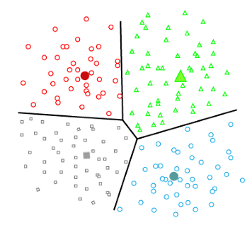Partitioning Clustering

2. Hierarchical Clustering

• Agglomerative (Bottom-Up): Starts with each data point as its own cluster and iteratively merges the closest clusters until only one cluster remains or the desired number of clusters is achieved.
  • Advantages: Does not require specifying the number of clusters in advance, provides a dendrogram for visualization.
  • Disadvantages: Computationally expensive, less efficient for large datasets.
• Divisive (Top-Down): Starts with all data points in one cluster and recursively splits them into smaller clusters.
  • Advantages: Can produce different levels of clustering granularity.
  • Disadvantages: Even more computationally expensive than agglomerative methods.

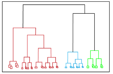Hierarchical Clustering

3. Density-Based Clustering

• DBSCAN (Density-Based Spatial Clustering of Applications with Noise): Forms clusters based on dense regions of data points. It can find arbitrarily shaped clusters and identify noise (outliers).
  • Advantages: Can find arbitrarily shaped clusters, robust to outliers, does not require specifying the number of clusters.
  • Disadvantages: Sensitive to the choice of parameters (epsilon and minPts), may struggle with varying densities.

Density-Based Clustering

4. Model-Based Clustering

• Gaussian Mixture Models (GMM): Assumes that the data is generated from a mixture of several Gaussian distributions. Uses the Expectation-Maximization (EM) algorithm to estimate the parameters.
  • Advantages: Can handle complex cluster shapes, provides a probabilistic assignment of data points to clusters.
  • Disadvantages: Requires specifying the number of clusters, can be computationally expensive.

5. Grid-Based Clustering

• STING (Statistical Information Grid): Divides the data space into a grid and performs clustering within each cell.
  • Advantages: Efficient for large datasets, less sensitive to the input order of data points.
  • Disadvantages: Quality of clustering depends on grid resolution.

6. Fuzzy Clustering

• Fuzzy C-Means: Each data point belongs to all clusters with varying degrees of membership, as opposed to hard assignments in K-Means.
  • Advantages: Provides more nuanced cluster assignments, useful for overlapping clusters.
  • Disadvantages: More complex and computationally intensive, requires specifying the number of clusters and fuzziness parameter.

Choosing the Right Clustering Method

Choosing the appropriate clustering method depends on the specific characteristics of the dataset and the goals of the analysis. Factors to consider include:

• Number of Clusters: Whether the number of clusters is known or needs to be determined.
• Cluster Shape: Whether clusters are expected to be spherical, elongated, or irregularly shaped.
• Noise and Outliers: The presence and importance of handling noise and outliers.
• Scalability: The size of the dataset and computational resources available.
• Interpretability: The need for interpretability and visualization of the clustering results.

Evaluating Clustering Results

Evaluating the quality of clustering results can be challenging since clustering is unsupervised. Common evaluation metrics include:

• Internal Measures: Evaluate the clustering based on the data itself, such as:
• Silhouette Score: Measures how similar a point is to its own cluster compared to other clusters.
• Davies-Bouldin Index: Considers the ratio of within-cluster distances to between-cluster distances.
• External Measures: Compare the clustering results to an external ground truth (if available), such as:
• Adjusted Rand Index (ARI): Measures the similarity between two data clusterings, considering all pairs of samples.
• Normalized Mutual Information (NMI): Measures the amount of shared information between the clustering and the ground truth.
• Visual Inspection: Plotting the data and visually inspecting the clusters can provide insights into their quality.

Clustering is a powerful technique for exploratory data analysis, enabling the discovery of patterns and structures within datasets. By understanding the different types of clustering methods and their applications, you can choose the best approach for your specific data and analysis needs.

 

Python Programming: Lists in Python

The sequence is the most fundamental data structure in Python. Every component in a series has an index, or location, assigned to it. Zero is the first index, one is the second, and so on. Although there are six built-in sequence types in Python, the most used ones are lists and tuples, which are what we’ll be working on in this article. All sequence kinds allow you to do specific tasks. Indexing, slicing, adding, multiplying, and membership checking are some of these operations. Furthermore, Python includes built-in functions for determining a sequence’s length as well as its greatest and smallest members.

Python Lists: A list of comma-separated values objects enclosed in square brackets is the most flexible datatype that Python has to offer. One important feature of a list is that its entries don’t have to be of the same kind. It’s easy to create a list by simply placing several values, separated by commas, between square brackets.

list1=[‘New York’, ‘New Delhi’, ‘Sydney’, ‘Totonto’, ‘Sania’]

list2=[20, 30, 34, 45, 55, 38]

How to Access Values in Lists: To retrieve values from lists, use the square brackets for slicing in conjunction with the index or indices to extract the value present at that index.

print(“list1[2]: “, list1[2])

print(“list2[2:4]: “, list2[2:4])

The output will be:

list1[2]: Sydney

list2[2:4]: [34,45]

Python Commands for Data Visualization

Python provides several powerful libraries for data visualization. Here are some commonly used Python libraries along with example commands to perform data visualization:

1. Matplotlib: Matplotlib is a versatile plotting library that provides a wide range of visualization options.

   import matplotlib.pyplot as plt

   # Line plot

   x = [1, 2, 3, 4, 5]

   y = [1, 4, 9, 16, 25]

   plt.plot(x, y)

   plt.xlabel('X-axis')

   plt.ylabel('Y-axis')

   plt.title('Line Plot')

   plt.show()

 

  # Bar plot

   labels = ['A', 'B', 'C']

   values = [10, 15, 7]

   plt.bar(labels, values)

   plt.xlabel('Categories')

   plt.ylabel('Values')

   plt.title('Bar Plot')

   plt.show()

  2. Seaborn: Seaborn is a statistical data visualization library built on top of Matplotlib. It provides a high-level interface for creating attractive and informative visualizations.

   import seaborn as sns

   # Scatter plot

   tips = sns.load_dataset('tips')

   sns.scatterplot(data=tips, x='total_bill', y='tip', hue='smoker')

   plt.xlabel('Total Bill')

   plt.ylabel('Tip')

   plt.title('Scatter Plot')

   plt.show()

  

 

 # Box plot

   sns.boxplot(data=tips, x='day', y='total_bill')

   plt.xlabel('Day')

   plt.ylabel('Total Bill')

   plt.title('Box Plot')

   plt.show()

3. Plotly: Plotly is an interactive plotting library that allows you to create interactive and dynamic visualizations.

   import plotly.graph_objects as go

   # Scatter plot

   fig = go.Figure(data=go.Scatter(x=[1, 2, 3, 4, 5], y=[1, 4, 9, 16, 25]))

   fig.update_layout(title='Scatter Plot', xaxis_title='X-axis', yaxis_title='Y-axis')

   fig.show()

 # Heatmap

   z = [[1, 2, 3], [4, 5, 6], [7, 8, 9]]

   fig = go.Figure(data=go.Heatmap(z=z))

   fig.update_layout(title='Heatmap')

   fig.show()

 

4. Pandas: Pandas is a powerful data analysis library that includes built-in visualization capabilities.

   import pandas as pd

   # Line plot

   df = pd.DataFrame({'x': [1, 2, 3, 4, 5], 'y': [1, 4, 9, 16, 25]})

   df.plot(x='x', y='y', kind='line')

   plt.xlabel('X-axis')

   plt.ylabel('Y-axis')

   plt.title('Line Plot')

   plt.show()

   

# Histogram

   df.plot(kind='hist');

   plt.xlabel('Values')

   plt.ylabel('Frequency')

   plt.title('Histogram')

   plt.show()

These are just a few examples of the vast possibilities for data visualization in Python. Each library offers a wide range of customization options, so you can tailor your visualizations to your specific needs.

Instance-Based Classification in Machine Learning

Instance-based classification, also known as instance-based learning or lazy learning, is a machine learning approach where the classification of new instances is based on the similarity to existing labeled instances in the training data. Instead of explicitly constructing a general model, instance-based classifiers store the training instances and use them directly during the classification process.

Here is a general overview of instance-based classification in machine learning:

1. Data Preparation: Gather and preprocess the data, as done in other classification tasks. Clean the data, handle missing values, and transform the features into a suitable format for similarity calculation.

2. Instance Storage: Store the labeled instances from the training data without explicitly constructing a model. The instances are typically stored in a data structure such as a k-d tree, hash table, or simply as a list of training instances.

3. Similarity Measure: Define a similarity measure to quantify the similarity between instances. Common similarity measures include Euclidean distance, cosine similarity, Hamming distance, or other domain-specific similarity metrics.

4. Classification Process:

• Nearest Neighbor Search: When a new instance needs to be classified, the instance-based classifier searches for the most similar instances in the stored training data based on the defined similarity measure. The number of nearest neighbors to consider is typically determined by a user-defined parameter (e.g., k nearest neighbors).
• Label Assignment: The class labels of the nearest neighbors are examined. The class label assigned to the new instance can be determined based on a majority vote of the neighbors' class labels (for classification tasks) or by averaging their labels (for regression tasks).
• Weighted Voting: Optionally, the contribution of each neighbor to the final classification decision can be weighted based on its similarity to the new instance. Closer neighbors may have more influence on the prediction than more distant ones.

5. **Model Evaluation:** Evaluate the performance of the instance-based classifier using appropriate evaluation metrics, such as accuracy, precision, recall, F1 score, or confusion matrix. These metrics measure the quality of the classification results compared to the ground truth labels.

Application areas of Instance-based classification

Instance-based classification has several advantages, including its ability to handle complex decision boundaries, flexibility in adapting to new data, and simplicity in training. It is particularly suitable for situations where the decision boundaries are nonlinear or when the distribution of the data is unknown. However, instance-based classifiers can be computationally expensive during the classification phase, especially when dealing with large training datasets. Common instance-based classifiers include k-nearest neighbors (k-NN), kernel density estimation, and case-based reasoning.

Bayesian classification in Machine Learning

Bayesian classification is a machine learning approach that applies the principles of Bayesian statistics to classify instances. It is based on Bayes' theorem, which provides a way to update probabilities based on new evidence. Bayesian classification models calculate the posterior probability of each class given the observed features and then assign the class label with the highest posterior probability.

Here is a general overview of Bayesian classification in machine learning:

1. Data Preparation: Gather and preprocess the data, as done in other classification tasks. Clean the data, handle missing values, and transform the features into a suitable format for the Bayesian classifier.

2. Model Training: In Bayesian classification, the model's parameters are estimated from the training data using the observed frequencies of features and class labels. The two main types of Bayesian classifiers are Naive Bayes and Bayesian Belief Networks (BBNs).

• Naive Bayes: The Naive Bayes classifier assumes independence between features given the class label. It calculates the conditional probability of each feature given each class and the prior probability of each class. The final classification is determined by combining the class priors and feature likelihoods using Bayes' theorem.
• Bayesian Belief Networks: BBNs are graphical models that represent dependencies between features and class labels using a directed acyclic graph. The conditional probabilities are specified in the graph, and inference is performed to calculate the posterior probabilities of the class labels given the observed features.

3. Model Evaluation: Evaluate the performance of the Bayesian classifier using appropriate evaluation metrics, such as accuracy, precision, recall, F1 score, or confusion matrix. These metrics measure the quality of the classification results compared to the ground truth labels.

4. Prediction: Once the Bayesian classifier is trained and evaluated, it can be used to make predictions on new, unseen data. The classifier calculates the posterior probability of each class given the observed features using Bayes' theorem and assigns the class label with the highest posterior probability.

Application areas in Bayesian classification

Bayesian classification offers several advantages, including its simplicity, efficiency in training and prediction, and ability to handle high-dimensional data. It can be particularly useful when dealing with small training datasets or when interpretability of the classification process is important. However, the Naive Bayes assumption of feature independence may not hold in some cases, which can lead to suboptimal results. Bayesian classification is commonly used in spam filtering, text categorization, sentiment analysis, and document classification tasks.

Rule-Based Classification in Machine Learning

Rule-based classification, also known as rule-based learning or rule-based classification modeling, is a machine learning approach that relies on explicitly defined rules to make predictions or classify instances. Instead of learning patterns and relationships from data, rule-based classifiers use predefined rules that are derived from human expertise or domain knowledge.

Here is a general overview of rule-based classification in machine learning:

1. Rule Generation: Create a set of rules based on human expertise or domain knowledge. These rules are typically in the form of "if-then" statements that specify conditions and corresponding actions or class labels. For example, a rule could be "if feature A is true and feature B is false, then assign class label X."

2. Data Preparation: Gather and preprocess the data, similar to other classification tasks. Clean the data, handle missing values, and transform the features into a suitable format for rule evaluation.

3. Rule Evaluation: Apply the generated rules to the input instances or data. Evaluate the conditions specified in each rule and check if they are satisfied or not. If a rule's conditions are met, the corresponding action or class label is assigned to the instance.

4. Rule Conflict Resolution: Handle situations where multiple rules are applicable to the same instance and may lead to conflicting predictions. Various strategies can be employed, such as giving priority to specific rules, considering the rule with the highest confidence, or using voting mechanisms.

5. Evaluation and Performance: Assess the performance of the rule-based classifier using appropriate evaluation metrics, such as accuracy, precision, recall, F1 score, or confusion matrix. These metrics measure the quality of the classification results compared to the ground truth labels.

6. Refinement and Rule Adaptation: Refine and adapt the rules based on feedback and performance evaluation. Domain experts or data analysts can analyze the classification results, identify shortcomings or inconsistencies in the rules, and modify or add new rules to improve the classifier's performance.

Application areas of Rule-based Classification:

Rule-based classification can be effective in certain scenarios, particularly when there is substantial domain knowledge available and the decision-making process can be explicitly defined. It is commonly used in expert systems, knowledge-based systems, and applications where interpretability and transparency of the decision-making process are crucial. Rule-based classifiers can be easily understood and verified, making them valuable in domains like medicine, finance, and law, where human expertise and interpretability are highly valued.

Probabilistic Classification in Machine Learning

Probabilistic classification, also known as probabilistic modeling or probabilistic classification modeling, is a machine learning approach that assigns probabilities to each class label instead of making deterministic predictions. It provides a measure of uncertainty and allows for more nuanced decision-making.

Here is a general overview of probabilistic classification in machine learning:

1. Data Preparation: Gather and preprocess the data, as done in other classification tasks. Clean the data, handle missing values, and transform the features into a suitable format for the learning algorithm.

2. Model Selection: Choose an appropriate probabilistic classification model. Popular models include Naïve Bayes, logistic regression, random forests with probability estimation, Gaussian processes, and probabilistic graphical models like Bayesian networks.

3. Model Training: Train the selected model using labeled data. During training, the model learns the underlying patterns and relationships between features and class labels. The goal is to estimate the parameters of the model that maximize the likelihood of the observed data.

4. Probabilistic Prediction: Once the model is trained, it can be used to make probabilistic predictions on new, unseen data. Instead of providing a deterministic prediction of the class label, the model assigns a probability or confidence score to each class label. The probabilities indicate the likelihood of an instance belonging to each class.

5. Decision Threshold: To make a binary decision, you can set a decision threshold on the predicted probabilities. For example, if the predicted probability for a class is above a certain threshold, it can be considered as the predicted class label. Otherwise, it can be considered as the other class label. The threshold can be adjusted based on the trade-off between precision and recall or other evaluation metrics.

6. Evaluation: Evaluate the performance of the probabilistic classification model using appropriate evaluation metrics. Common metrics include log loss, Brier score, area under the receiver operating characteristic (ROC) curve, precision-recall curve, and calibration plots. These metrics measure the quality of the predicted probabilities and the accuracy of the probabilistic predictions.

7. Model Calibration: Probabilistic classification models may need calibration to ensure that the predicted probabilities are well-calibrated, meaning that they reflect the true likelihood of an instance belonging to a class. Calibration techniques such as Platt scaling or isotonic regression can be applied to adjust the predicted probabilities.

Application areas of Probabilistic classification:

Probabilistic classification is valuable in various machine learning applications, especially when decision-making requires a measure of uncertainty. It is widely used in spam filtering, sentiment analysis, medical diagnosis, credit risk assessment, anomaly detection, and many other domains where understanding the confidence of predictions is essential.