PREPARE DATA FOR MACHINE LEARNING

When utilizing ML to address real-world issues, data preparation is typically the initial step. This is due to the fact that before a dataset can be used to train machine learning or deep learning algorithms, it usually contains a number of inconsistencies that must be fixed. The following is a list of problems with unprepared data:

• Missing Values in the Dataset
• Different File Formats
• Outlying Data Points
• Inconsistency in variable values
• Irrelevant feature variables

STEPS INVOLVED IN DATA PREPARATION ARE AS FOLLOWS:

1. Gather data

Finding the appropriate data is the first step in the data preparation process. This might originate from a database that already exists or could be added on the fly.

2. Discover and assess data

Discovering each dataset is crucial after data collection. Understanding the data and what has to be done before the data is relevant in a given context are the goals of this step.

3. Cleanse and validate data

Though generally, the most time-consuming step in the data preparation process, cleaning up the data is essential for eliminating inaccurate data and filling in any gaps. Here, crucial duties include:

• Eliminating irrelevant information and outliers, Adding values when there are gaps Data standardization, data masking, and sensitive or private data entry

4. Transform and enrich data

Data transformation involves changing the format or value entries to achieve a specific result or to make the data more comprehensible to a larger audience. Adding to and connecting data with additional relevant information in order to deliver deeper insights is referred to as enriching data.

5. Store data

When the data is ready, it can be saved or sent to a third-party program, like a business intelligence tool, opening the door for processing and analysis.

Step 1: Importing pandas as pd in python to use this library

import pandas as pd

import numpy as np

Step 2:  Reading data in excel/csv file

df=pd.read_csv('father-son.csv')
df

df.describe()

Step 2: Splitting dataset into Training and Test datasets

from sklearn.model_selection import train_test_split

X = df.drop("Son", axis=1)

y = df['Son']

X_train,X_test,y_train,y_test= train_test_split(X,y, test_size = 0.2,\

                                                   random_state=112)

from sklearn.linear_model import LinearRegression

my_model = LinearRegression() 

result = my_model.fit(X_train, y_train) 

predictions = result.predict(X_test) 

plt.scatter(X_train, y_train, color ='c') 

plt.plot(X_test, predictions, color ='k') 

plt.show()

from sklearn.metrics import r2_score

r2_score(y_test,predictions)

import numpy as np

from sklearn import metrics

print ('MAE: ', metrics.mean_absolute_error(y_test, predictions))

print ('MSE: ',metrics.mean_squared_error(y_test, predictions))

print ('RMSE: ',np.sqrt(metrics.mean_squared_error(y_test, predictions)))

import seaborn as sns

sns.jointplot(df['Father'], df['Son'])

sns.jointplot(x='Father', y='Son', data = df, kind = 'hex')

sns.pairplot(df)

Introduction to Python Programming

Python is a high-level, interpreted programming language known for its simplicity and readability. Created by Guido van Rossum and first released in 1991, Python has become one of the most popular programming languages in the world. It is widely used in various fields, from web development and data science to artificial intelligence and automation.

Why Choose Python?

Python’s design philosophy emphasizes code readability and simplicity, making it an ideal choice for both beginners and experienced developers. Here are some reasons why Python stands out:

1. Ease of Learning: Python’s syntax is clear and straightforward, closely resembling the English language. This makes it easier to learn and write code.
2. Versatility: Python is a general-purpose language, which means it can be used to build a wide variety of applications, including web applications, desktop applications, games, and more.
3. Extensive Libraries and Frameworks: Python boasts a rich ecosystem of libraries and frameworks that simplify development tasks. For example, Django and Flask for web development, NumPy and pandas for data analysis, and TensorFlow and PyTorch for machine learning.
4. Community Support: Python has a large and active community, which means you can find plenty of resources, tutorials, and forums to help you solve problems and learn new skills.
5. Integration Capabilities: Python can easily integrate with other languages and technologies, making it a versatile tool in a developer’s toolkit.

Key Features of Python

• Interpreted Language: Python is an interpreted language, meaning that your code is executed line by line. This allows for quick testing and debugging.
• Dynamic Typing: Python uses dynamic typing, so you don’t need to declare the data type of a variable when you create one. This flexibility can speed up development.
• Object-Oriented: Python supports object-oriented programming (OOP), which allows you to create classes and objects, enabling code reuse and modularity.
• High-Level Language: Python abstracts away most of the complex details of the computer’s hardware, allowing you to focus on programming logic rather than low-level details.
• Cross-Platform: Python is cross-platform, meaning it runs on various operating systems, including Windows, macOS, and Linux, without requiring modification.

Python’s Role in Modern Development

Python has cemented its role in modern development due to its applicability in emerging fields:

• Data Science and Analytics: Python’s data manipulation and visualization libraries like pandas, Matplotlib, and Seaborn have made it a staple in data science.
• Machine Learning and Artificial Intelligence: Libraries like TensorFlow, Keras, and Scikit-Learn have enabled Python to become a leading language in AI and machine learning development.
• Web Development: Frameworks like Django and Flask have simplified the creation of robust and scalable web applications.
• Automation and Scripting: Python’s simplicity makes it an excellent choice for writing scripts to automate repetitive tasks.

Getting Started with Python

To start programming in Python, you’ll need to set up your development environment:

1. Install Python: Download and install the latest version of Python from the official website (python.org).
2. Choose an Integrated Development Environment (IDE): Popular choices include PyCharm, VSCode, and Jupyter Notebook. These tools provide features like syntax highlighting, debugging, and project management.
3. Write Your First Program: Open your IDE and write a simple “Hello, World!” program to get a feel for Python’s syntax.

1	print("Hello, World!")

Conclusion

Python is a powerful and versatile language that can open doors to numerous opportunities in various fields. Whether you’re a beginner looking to learn your first programming language or an experienced developer exploring new domains, Python provides the tools and resources you need to succeed.

How to handle Outliers

Handling outliers in a dataset is an important step in data preprocessing to ensure that extreme values do not adversely affect the performance and accuracy of machine learning models. Here are some common approaches to handling outliers:

1. Detecting outliers:

• Visual inspection: Plotting the data using box plots, scatter plots, or histograms can help identify outliers visually.
• Statistical methods: Use statistical techniques such as z-scores, interquartile range (IQR), or modified z-scores to detect outliers based on their deviation from the mean or median.

2. Handling outliers:

• Removing outliers: If the outliers are due to data entry errors or represent extreme anomalies, it might be appropriate to remove them from the dataset. However, this should be done with caution, as removing too many outliers can lead to the loss of valuable information.
• Transforming data: Applying mathematical transformations such as logarithmic, square root, or reciprocal transformations can help make the data more normally distributed and reduce the impact of outliers.
• Winsorizing: Winsorization involves replacing extreme outlier values with less extreme values. For example, capping the outliers at a certain percentile (e.g., replacing values above the 99th percentile with the 99th percentile value).
• Binning: Grouping continuous data into bins or intervals can help reduce the impact of outliers. Instead of using the raw values, you can assign the data points to the corresponding bin.
• Imputation: If the outliers are due to missing values, imputation techniques such as mean, median, or regression-based imputation can be used to replace the outliers with plausible values.
• Model-based approaches: Some machine learning algorithms are robust to outliers, such as robust regression or decision tree-based models. In such cases, using models that can handle outliers effectively might be a suitable approach.

It's important to note that the choice of handling outliers depends on the specific dataset, the nature of the outliers, and the objectives of the analysis. It is advisable to carefully evaluate the impact of outlier handling on the overall data distribution and the downstream analysis or modeling tasks.

Additionally, it's crucial to document and report the handling of outliers in your analysis to ensure transparency and reproducibility.

Machine Learning Algorithms : Python Vs. R

Linear Regression

Using Python

#Import all necessary libraries like pandas,numpy etc.

from sklearn import linear_model

#Load Train and Test datasets

#Identify feature(s) and response variable(s) and values must be numeric and numpy arrays 

X_train=input_variables_values_training_datasets 

y_train=target_variables_values_training_datasets 

x_test=input_variables_values_test_datasets

#Create linear regression object

linear = linear_model.LinearRegression ()

#Train the model using the training sets and check score 

linear.fit(X_train, y_train) 

linear.score(X_train, y_train)

#Equation coefficient and Intercept

print('Coefficient: In', linear.coef_)

print('Intercept: \n', linear.intercept_)

#Predict Output 

predicted= linear.predict(x_test)

Using R

#Load Train and Test datasets

#Identify feature and response variable(s) and values must be numeric and numpy arrays 

X_train <- input_variables_values_training_datasets 

y_train <- target_variables_values_training_datasets 

x_test ‹- input variables values test datasets 

x <-cbind(x_train,y_train)

#Train the model using the training sets and check score

linear <- lm(y_train ~ ., data = x)

summary (linear)

#Predict Output

predicted= predict (linear, x_test)

Basic Git Commands cheat sheet

 

git config

Syntax: git config –global user.name “[name]”

Syntax: git config –global user.email “[email address]”

This command sets the author name and email address respectively to be used with your commits.

git init

Syntax: git init [repository name]

This command is used to start a new repository.

git add

Syntax: git add [file]

This command adds a file to the staging area.

Syntax: git add *

This command adds one or more to the staging area.

git clone

Syntax: git clone [url]

This command is used to obtain a repository from an existing URL.

git commit

Syntax: git commit -m “[ Type any commit message of your choice]”

This will record or snapshot the file permanently in the version history.

Syntax: git commit -a

This will commit any files you’ve added with the git add command and also will commit any files you’ve changed since then.

git reset

Syntax: git reset [file]

This command unstages the file, but it saves/preserves the file contents.

Syntax: git reset [commit]

This command undoes all the commits after the specified commit and preserves the changes locally.

Syntax: git reset –hard [commit]

This command discards all history and goes back to the specified commit.

git status

Syntax: git status

This command lists all the files that have to be committed.

git show

Syntax: git show [commit]

This command shows the metadata and content changes of the specified commit.

git branch

Syntax: git branch

This command lists all the local branches in the current repository.

Syntax: git branch [branch name]

This command creates a new branch.

Syntax: git branch -d [branch name]

This command deletes the feature branch.

git checkout

Syntax: git checkout [branch name]

This command is used to switch from one branch to another.

Syntax: git checkout -b [branch name]

This command creates a new branch and also switches to it.

git remote

Syntax: git remote add [variable name] [Remote Server Link]

This command is used to connect your local repository to the remote server.

git push

Syntax: git push [variable name] master

This command sends the committed changes of master branch to your remote repository.

Syntax: git push [variable name] [branch]

This command sends the branch commits to your remote repository.

Syntax: git push –all [variable name]

This command pushes all branches to your remote repository.

Syntax: git push [variable name] :[branch name]

This command deletes a branch on your remote repository.

git pull

Syntax:  git pull [Repository Link]

This command fetches and merges changes on the remote server to your working directory.

git tag

Syntax: git tag [commitID]

This command is used to give tags to the specified commit.

git merge

Syntax: git merge [branch name]

This command merges the specified branch’s history into the current branch.

Types of Error in Statistics

A statistical error, in simple words, is the difference between a measured value and the actual value of the data that was gathered.

A hypothesis test can result in two types of errors.

1. Type 1 error

2. Type 2 error

Type 1 Error: A Type-I error occurs when sample results reject the null hypothesis despite being true.

Type 2 Error: A Type-II error occurs when the null hypothesis is not rejected when it is false.

In other words, In statistics, a Type I error is a false positive conclusion, while a Type II error is a false negative conclusion.

The significance level, or alpha (), determines the likelihood of a Type I error, whereas beta () determines the likelihood of a Type II error. These risks can be reduced by carefully designing the layout of your study.

Example: Type I vs Type II error:

You have mild symptoms of COVID-19 and your doctor advised you to go for a test. The following two errors could potentially occur:

Type I error (false positive): the test result says you are COVID positive, but you actually don’t.

Type II error (false negative): the test result says you are COVID negative, but you actually do

What is Confusion Matrix?

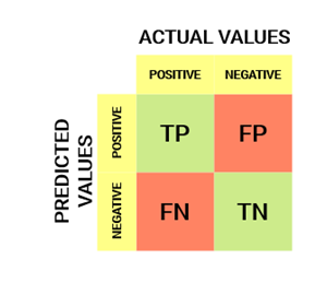
An N x N matrix called a confusion matrix is used to assess the effectiveness of a classification model, where N is the total number of target classes. In the matrix, the actual goal values are contrasted with those that the machine learning model anticipated. This provides us with a comprehensive understanding of the classification model's performance and the types of mistakes it is making.

A 2 x 2 matrix with 4 values is what we would have for a binary classification problem:

Now let's interpret the matrix:

• Positive or negative values can be assigned to the target variable.

The target variable's actual values are shown in the columns, while its anticipated values are shown in the rows.

True Positive (TP): When the model's predicted value matches the actual value and the actual value was positive.

True Negative (TN): When the model's prediction and the observed value coincide. When the observed value was negative and the model had anticipated a negative value.

Type 1 error: False Positive (FP)

Also known as the Type 1 mistake, this error occurs when the anticipated value is incorrectly forecasted, the actual value is negative, while the model projected a positive value.

Type 2 error: False Negative (FN)

Also known as the Type 2 error, these conditions include: the predicted value was incorrectly forecasted; the actual value was positive although the model projected a negative value; and

To help you grasp this better, let's use an example. Consider a classification dataset that contained 10000 data points. We apply a classifier to it and obtain the confusion matrix shown below:

The Confusion matrix's various values would be as follows:

True Positive (TP) = 6500, indicating that the model accurately categorised 6500 positive class data points.

True Negative (TN) = 2300, indicating that the model properly identified 2300 data points in the negative class.

False Positive (FP) = 700, which means that the model misclassified 700 negative class data points as being in the positive class.

500 positive class data points were mistakenly assigned to the negative class by the model, resulting in 500 false negatives (FN)

Evaluation parameters

1. Accuracy
2. Precision
3. Recall
4. F1-Score

The following are the evaluation parameters considered:

Accuracy: The number of all accurate predictions divided by the overall dataset size yields accuracy (ACC). The accuracy ranges from 0.0 to 1.0, with 1.0 being the best. You can alternatively calculate it by using 1 - ERR.

Technically, Accuracy is calculated as the total number of two correct predictions (TP + TN) divided by the total number of a dataset (P + N).

Accuracy=(TP+TN)/(TP+FP+FN+TN)

Precision: Precision is an evaluation metric that combines relevant and successfully retrieved items over all of the results that were successfully obtained. When the likelihood of a false-positive prediction is large, it is mostly employed.

Precision (TNR) = TP/(TP+FP)

Recall: Recall is a measure when a False negative is considered.

Recall (Sensitivity or TPR) = TP/(TP+FN)

F1-Score: F1-Score is an evaluation technique that maintains a balance between precision and recall.

F1-Score = 2 * (Precision*Recall)/(Precision+Recall)

What is the Purpose of a Confusion Matrix?

Let's consider a classification issue before we respond to this query.

Consider the scenario where you want to segregate those who are infected with an infectious virus from the healthy population before they begin to exhibit symptoms. Our goal variable would have the following two values: Sick and Not Sick.

You're probably thinking why we need a confusion matrix when we already have Accuracy, our go-to companion in any situation. Let's see where accuracy falls short.

Let's take an example of an unbalanced dataset. The negative class has 947 data points, while the positive class has only three. We'll calculate the accuracy as follows: