Tuesday, December 14, 2021

Basic Git Commands cheat sheet


git config

Syntax: git config –global user.name “[name]”

Syntax: git config –global user.email “[email address]”

This command sets the author name and email address respectively to be used with your commits.

git init

Syntax: git init [repository name]

This command is used to start a new repository.

git add

Syntax: git add [file]

This command adds a file to the staging area.

Syntax: git add *

This command adds one or more to the staging area.

git clone

Syntax: git clone [url]

This command is used to obtain a repository from an existing URL.

git commit

Syntax: git commit -m “[ Type any commit message of your choice]”

This will record or snapshot the file permanently in the version history.

Syntax: git commit -a

This will commit any files you’ve added with the git add command and also will commit any files you’ve changed since then.

git reset

Syntax: git reset [file]

This command unstages the file, but it saves/preserves the file contents.

Syntax: git reset [commit]

This command undoes all the commits after the specified commit and preserves the changes locally.

Syntax: git reset –hard [commit]

This command discards all history and goes back to the specified commit.

git status

Syntax: git status

This command lists all the files that have to be committed.

git show

Syntax: git show [commit]

This command shows the metadata and content changes of the specified commit.

git branch

Syntax: git branch

This command lists all the local branches in the current repository.

Syntax: git branch [branch name]

This command creates a new branch.

Syntax: git branch -d [branch name]

This command deletes the feature branch.

git checkout

Syntax: git checkout [branch name]

This command is used to switch from one branch to another.

Syntax: git checkout -b [branch name]

This command creates a new branch and also switches to it.

git remote

Syntax: git remote add [variable name] [Remote Server Link]

This command is used to connect your local repository to the remote server.

git push

Syntax: git push [variable name] master

This command sends the committed changes of master branch to your remote repository.

Syntax: git push [variable name] [branch]

This command sends the branch commits to your remote repository.

Syntax: git push –all [variable name]

This command pushes all branches to your remote repository.

Syntax: git push [variable name] :[branch name]

This command deletes a branch on your remote repository.

git pull

Syntax:  git pull [Repository Link]

This command fetches and merges changes on the remote server to your working directory.

git tag

Syntax: git tag [commitID]

This command is used to give tags to the specified commit.

git merge

Syntax: git merge [branch name]

This command merges the specified branch’s history into the current branch.
Types of Error in Statistics


A statistical error, in simple words, is the difference between a measured value and the actual value of the data that was gathered.

A hypothesis test can result in two types of errors.

1. Type 1 error

2. Type 2 error


Type 1 Error: A Type-I error occurs when sample results reject the null hypothesis despite being true.

Type 2 Error: A Type-II error occurs when the null hypothesis is not rejected when it is false.


In other words, In statistics, a Type I error is a false positive conclusion, while a Type II error is a false negative conclusion.

The significance level, or alpha (), determines the likelihood of a Type I error, whereas beta () determines the likelihood of a Type II error. These risks can be reduced by carefully designing the layout of your study.

Example: Type I vs Type II error:

You have mild symptoms of COVID-19 and your doctor advised you to go for a test. The following two errors could potentially occur:

Type I error (false positive): the test result says you are COVID positive, but you actually don’t.

Type II error (false negative): the test result says you are COVID negative, but you actually do

Thursday, December 9, 2021

What is Confusion Matrix?

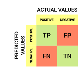
An N x N matrix called a confusion matrix is used to assess the effectiveness of a classification model, where N is the total number of target classes. In the matrix, the actual goal values are contrasted with those that the machine learning model anticipated. This provides us with a comprehensive understanding of the classification model's performance and the types of mistakes it is making.

A 2 x 2 matrix with 4 values is what we would have for a binary classification problem:

Now let's interpret the matrix:

• Positive or negative values can be assigned to the target variable.

The target variable's actual values are shown in the columns, while its anticipated values are shown in the rows.

True Positive (TP): When the model's predicted value matches the actual value and the actual value was positive.
True Negative (TN): When the model's prediction and the observed value coincide. When the observed value was negative and the model had anticipated a negative value.

Type 1 error: False Positive (FP)
Also known as the Type 1 mistake, this error occurs when the anticipated value is incorrectly forecasted, the actual value is negative, while the model projected a positive value.

Type 2 error: False Negative (FN)

Also known as the Type 2 error, these conditions include: the predicted value was incorrectly forecasted; the actual value was positive although the model projected a negative value; and

To help you grasp this better, let's use an example. Consider a classification dataset that contained 10000 data points. We apply a classifier to it and obtain the confusion matrix shown below:

The Confusion matrix's various values would be as follows:

True Positive (TP) = 6500, indicating that the model accurately categorised 6500 positive class data points.

True Negative (TN) = 2300, indicating that the model properly identified 2300 data points in the negative class.

False Positive (FP) = 700, which means that the model misclassified 700 negative class data points as being in the positive class.

500 positive class data points were mistakenly assigned to the negative class by the model, resulting in 500 false negatives (FN)

Evaluation parameters

  1. Accuracy
  2. Precision
  3. Recall
  4. F1-Score
The following are the evaluation parameters considered:

Accuracy: The number of all accurate predictions divided by the overall dataset size yields accuracy (ACC). The accuracy ranges from 0.0 to 1.0, with 1.0 being the best. You can alternatively calculate it by using 1 - ERR.
Technically, Accuracy is calculated as the total number of two correct predictions (TP + TN) divided by the total number of a dataset (P + N).

Accuracy=(TP+TN)/(TP+FP+FN+TN)

Precision: Precision is an evaluation metric that combines relevant and successfully retrieved items over all of the results that were successfully obtained. When the likelihood of a false-positive prediction is large, it is mostly employed.
Precision (TNR) = TP/(TP+FP)

Recall: Recall is a measure when a False negative is considered.

Recall (Sensitivity or TPR) = TP/(TP+FN)

F1-Score: F1-Score is an evaluation technique that maintains a balance between precision and recall.

F1-Score = 2 * (Precision*Recall)/(Precision+Recall)


What is the Purpose of a Confusion Matrix?

Let's consider a classification issue before we respond to this query.

Consider the scenario where you want to segregate those who are infected with an infectious virus from the healthy population before they begin to exhibit symptoms. Our goal variable would have the following two values: Sick and Not Sick.

You're probably thinking why we need a confusion matrix when we already have Accuracy, our go-to companion in any situation. Let's see where accuracy falls short.

Let's take an example of an unbalanced dataset. The negative class has 947 data points, while the positive class has only three. We'll calculate the accuracy as follows:


Wednesday, November 24, 2021

Classification in Supervised Machine Learning

Finding a function to divide the dataset into classes based on several parameters is the process of classification. In classification, data is divided into various classes by a computer program that has been trained on the training dataset.

Finding the mapping function to convert the input (x) to the discrete output is the goal of the classification algorithm (y).

Example: Email spam detection offers the clearest illustration of the Classification issue. When a new email arrives, the model determines whether it is spam or not based on training data from millions of emails on various parameters. The email gets placed in the Spam folder if it is considered spam.

What is Classification?

On the basis of training data, the Classification algorithm is a Supervised Learning technique that is used to categorize new observations. In classification, a program makes use of the dataset or observations that are provided to learn how to categorize/classify fresh observations into various classes or groups. For instance, Animal or Bird, Male or Female, Yes or No, 0 or 1, Spam or Not Spam. Targets, labels, or categories can all be used to describe classes.


Tuesday, November 23, 2021

Types of Regression

Regression comes in a variety of forms, and they are employed in data science and machine learning. The significance of each type varies depending on the situation, but fundamentally, all regression techniques examine the impact of the independent variable on the dependent variables. Here, we'll talk about a few significant types of regression, which are listed below:


  • Linear Regression
  • Logistic Regression
  • Support Vector Regression
  • Generalized Linear Models

Wednesday, November 17, 2021

Case Study: Working withTitanic Dataset

import pandas as pd

import numpy as np

import matplotlib.pyplot as plt

import seaborn as sns

df=pd.read_csv('titanic_dataset.csv') 

 #dataset can be downloaded from www.kaggle.com

df


df.head() # to show top 5 rows

df.tail(2) # to show bottom 2 rows

df.nunique()

df['Survived'].unique()

s1=df['Survived'].unique()df['Survived'].value_counts() # to find number of people survived vs not survived

#using matplotlib

plt.bar(s1.index,s1.values)

plt.show()


plt.bar(['Not Survived','Survived'],s1.values)

plt.show()


#seaborn method

sns.countplot(x='Survived', data=df)

plt.show()


df['Sex'].value_counts() # to find number of people survived vs not survived

s1

#seaborn method

sns.countplot(x='Sex', data=df)

plt.show()


df['Survived']==1

df[df['Survived']==1]

df[df['Survived']==1]['Sex'].value_counts()


df.groupby(['Survived']).sum()


df.groupby(['Survived','Sex']).size()

sns.catplot(x='Survived',hue='Sex',kind='count',data=df)

plt.show()


#dealing with missing values

df.isnull()

mean_age=df['Age'].mean()

mean_age

29.69911764705882

df['Age']=df['Age'].fillna(mean_age)

sns.kdeplot(df['Age'])


Saturday, November 13, 2021

Implementation of Machine Learning using Python

 # General Changes

# 1. Labeling the x-axis and y-axis

# 2. Title of the Graph

# 3. Figure Size

# 4. Annotate on the graph

# 5. Scale of the graph

# 6. Grid on the graph


import matplotlib.pyplot as plt

import numpy as np

plt.figure(figsize=(10,3))

x=np.array([10,30,45,67,90])

y=np.array([12,56,27,36,67])

for i in range(len(x)):

    plt.text(x[i],y[i],(x[i],y[i]))

for i in range(len(x)):

    plt.text(x[i],y[i],f'   ({x[i]},{y[i]})')


plt.plot(x,y,color='r',ls='--',lw=3,marker='*',ms=20,markeredgecolor='g')

plt.title('Height-Weight Graph',fontsize=20,fontweight='bold')

plt.xlim(-10,100)

plt.ylim(0,70)

plt.xlabel('X-axis values')

plt.ylabel('Y-axis values')

plt.grid()

plt.xticks(np.arange(-10,101,10))

plt.savefig("mylineplot.png")

plt.show()


# Take a numpy array named person and give 3 names for the same

# Take another numpy array named height and give their respective heights

# Plot a bar graph indicating the same

person = np.array([ 'Mr A', 'Mr B', 'Mr C' ])
height = np.array( [145,146,1351])
weight=np.array([45,56,47])                   
plt.bar(person,height,width=-0.4,align='edge',color='r',label='height')
plt.bar(person,weight,width=0.4,align='edge',color='g',label='weight')
plt.legend()
plt.xlabel('Person Name')
plt.ylabel ('Height in cms')
plt.show()


cities=np.array(['Mumbai', 'Bangalore','Ahemdabad','Delhi' ])

cities = np.array(['Mumbai','Bangalore','Ahmedabad','Delhi'])
population = np.array([12442373,8443675,5577940,11034555])
plt.pie(population,explode=[0,0.1,0,0],labels=cities,autopct='%.2f%%')
plt.show()


Saturday, November 6, 2021

Regression Analysis in Machine Learning

Regression analysis in supervised learning, uses one or more independent variables to describe the relationship between a dependent (target) and independent (predictor) variables. More specifically, regression analysis enables us to comprehend how, while other independent variables are held constant, the value of the dependent variable changes in relation to an independent variable. It forecasts real, continuous values like temperature, age, salary, and cost, among others.

We can understand the concept of regression analysis using the below example:

Example: Suppose there is a marketing company A, who does various advertisements every year to increase their sales based on that. The below list shows the advertisement made by the company in the last 10 years and the corresponding sales


The company is looking for a sales forecast for this year to plan an Rs. 150000 campaign for 2021. Regression analysis is therefore required in order to handle these kinds of prediction problems in machine learning.

Definition: Regression is a supervised learning method that enables us to predict the continuous output variable based on one or more predictor variables and aids in determining the correlation between variables. It is mostly used for forecasting, time series modeling, prediction, and establishing the causal connection between variables


Regression analysis-related terminologies: 

o Dependent Variable: In a regression study, the primary variable that we wish to predict or comprehend is referred to as the dependent variable. It also goes by the name target variable.

o Independent Variable: Also known as a predictor, independent variables are the elements that have an impact on the dependent variables or that are used to forecast their values.

o Outliers: An observation that deviates significantly from the norm in terms of either very low or very high values An outlier should be avoided as it might hurt the outcome.

o Multicollinearity: This situation is characterized by the independent variables having a higher correlation with one another than with other variables. It shouldn't be included in the dataset because it causes issues when determining which variable has the greatest impact.

o Overfitting and Underfitting: An overfitting problem occurs when our system performs well on the training dataset but poorly on the test dataset. Underfitting is the term used when an algorithm does not perform well even with training data.

INTRODUCTION TO MACHINE LEARNING

Machine Learning was first defined by Arthur Samuel in early 90's describing it as,” A field of study that gives the ability to the computer for self-learn without being explicitly programmed”, that means giving machines information without hard-coding it.

"A computer program is said to learn from experience E with respect to some class of tasks T and performance measure P if its performance at tasks in T, as measured by P, improves with experience E." - Tom Mitchell

Machine learning focuses on data-driven learning based on actual interactions and is the process of teaching computers and digital devices to learn and carry out tasks the same way humans do.

Machine learning (ML), a subset of the widely adopted idea of Artificial Intelligence (AI), transforms data into knowledge for programs and applications that provide computers the ability to do human-like tasks. This data helps machines function better over time and increases their accuracy all the while.

Types of Machine Learning:

Machine Learning can be broadly classified as:


  • Supervised Machine Learning: Supervised learning is most often employed category of machine learning. In this learning, labeled data is used to train the machine learning algorithm. Such algorithm uses labeled samples to predict future events by applying knowledge from the past to fresh data. The weights are adjusted until the model is well fitted when input data is inputted into it. Regression and classification algorithms are used in supervised learning to make predictions or divide data into distinct classes.
  • Unsupervised Machine Learning: Unsupervised machine learning includes building models using data without labels or clearly stated outcomes. These algorithms look for concealed patterns or data clusters without human interaction. As this method may identify same and different patterns in data, it is useful for exploratory data analysis, consumer segmentation, cross-selling strategies, and the finding of images and patterns. Clustering and association techniques are utilized to implement the models in unsupervised learning.
  • Semi-Supervised Machine Learning: This learning falls in between supervised and unsupervised learning. It uses a small amount of labeled dataset during training in order to manage feature selection or extraction and classification from a larger set of unlabeled data. Semi-supervised learning can be used to provide a best solution to the problem of not having enough labeled data. It also helps in case of labeling more data which would be beneficial but too expensive.


Clustering in Machine Learning

Clustering is a type of unsupervised learning in machine learning where the goal is to group a set of objects in such a way that objects in...